Activation And Loss Functions In Deep Learning

A network can run perfectly, produce tensors of the expected shape, and still be mathematically incapable of learning the task you gave it. A ReLU output may be asked to behave like a probability. A softmax may be used where several labels can be true. A loss may quietly expect logits while receiving probabilities.

Activation functions and loss functions do different jobs, but those jobs meet at the output layer. An activation changes a representation; a loss turns predictions and targets into the objective used for training. Choosing them together prevents a surprising number of silent mistakes.

Activation Functions

1. ReLU

\operatorname{ReLU}(x)=\max(0,x)

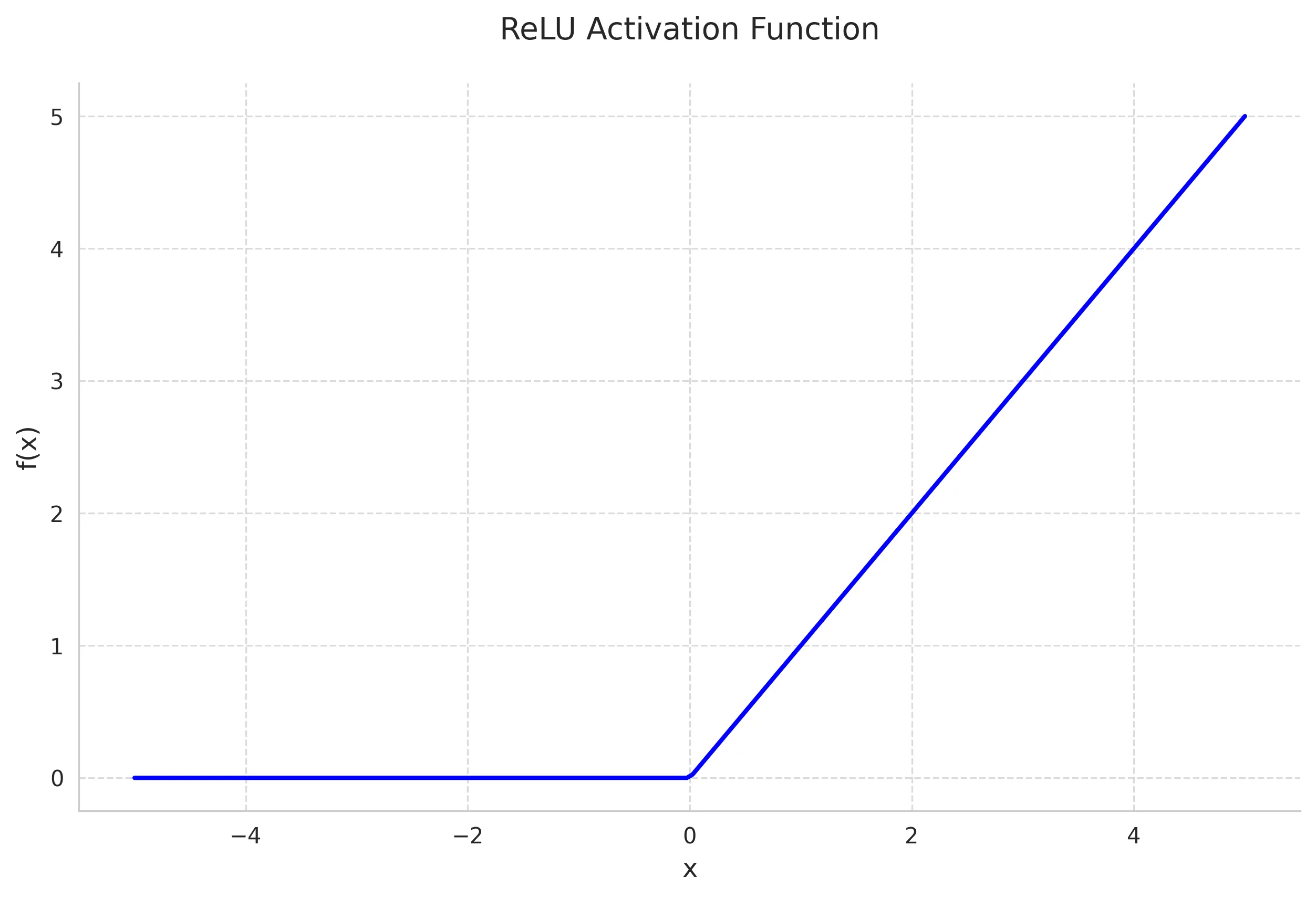
For $x\ne0$ :

\operatorname{ReLU}'(x)= \begin{cases} 1 & x>0\\ 0 & x<0 \end{cases}

At zero, frameworks choose a convenient subgradient, usually 0. ReLU is cheap and keeps a non-saturating derivative on its positive side. It does not guarantee that half the units will be active, and a unit that receives only negative pre-activations can stop learning.

Typical use: hidden layers in convolutional and dense networks.

2. Leaky ReLU

f(x)= \begin{cases} x & x>0\\ \alpha x & x\le0 \end{cases}

Leaky ReLU keeps a small derivative on the negative side. This reduces the risk of permanently inactive units but does not make it impossible. Parametric ReLU learns $\alpha$ rather than fixing it.

Typical use: a ReLU alternative when negative-side gradient flow helps.

3. Sigmoid

\sigma(x)=\frac{1}{1+e^{-x}}

\sigma'(x)=\sigma(x)(1-\sigma(x))

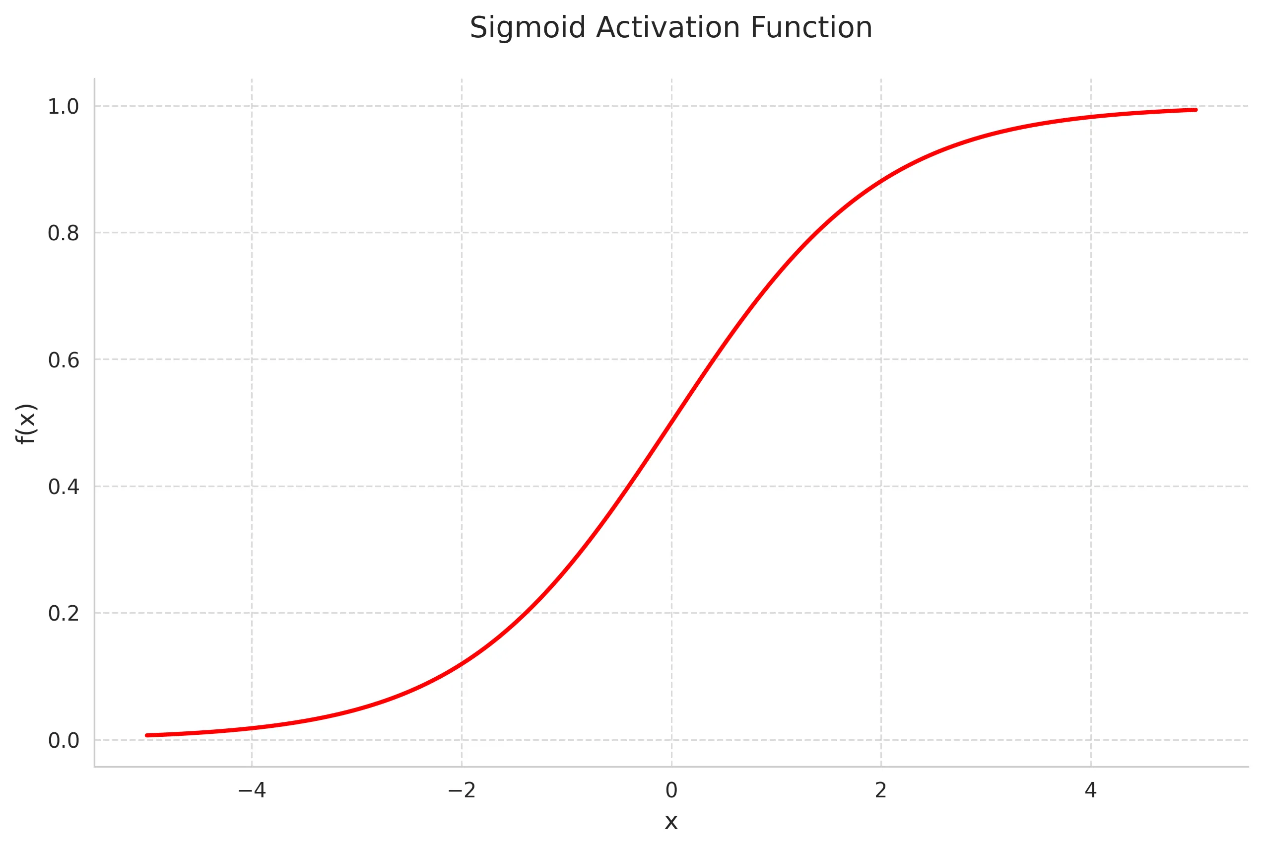
Sigmoid maps a logit to $(0,1)$ and is a natural output transformation for a binary event or independent multilabel targets. A number in this range can be interpreted as a model probability, but it is not automatically calibrated. Calibration has to be checked on representative held-out data.

Large positive or negative inputs saturate the function and produce small derivatives. For that reason, sigmoid is less common in ordinary hidden layers.

4. Tanh

\tanh(x)=\frac{e^x-e^{-x}}{e^x+e^{-x}}

\frac{d}{dx}\tanh(x)=1-\tanh^2(x)

Tanh is zero-centered and maps to $(-1,1)$ , but it also saturates at large magnitudes. In recurrent networks it is commonly used for candidate values and hidden-state updates, while sigmoid usually controls the gates themselves. It also appears in small networks where a bounded output is useful.

5. Softmax

Softmax converts logits into a categorical distribution

For logits $z_1,\ldots,z_K$ :

\operatorname{softmax}(z)_i= \frac{e^{z_i}}{\sum_{j=1}^{K}e^{z_j}}

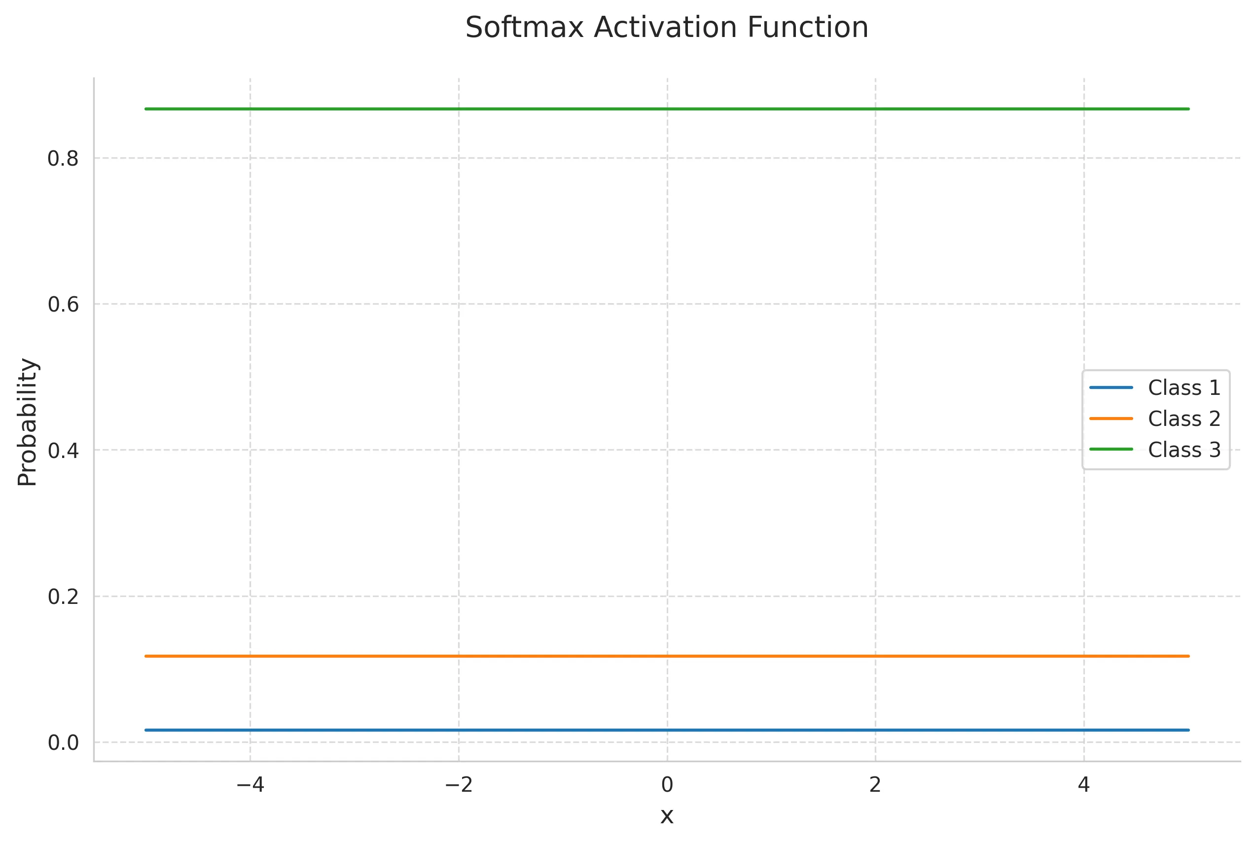
The outputs are positive and sum to one. The full Jacobian is:

\frac{\partial s_i}{\partial z_j}=s_i(\delta_{ij}-s_j)

This covers both cases: $s_i(1-s_i)$ when $i=j$ and $-s_is_j$ otherwise.

For numerical stability, compute exp(z - max(z)), or use a library function. During training, prefer a cross-entropy operation that accepts logits so the framework can combine log-softmax and negative log-likelihood stably.

Typical use: one-of- $K$ classification. It is not appropriate when several labels may be true independently; use one sigmoid per label for that case.

6. ELU

f(x)= \begin{cases} x & x>0\\ \alpha(e^x-1) & x\le0 \end{cases}

ELU has negative outputs and a smooth negative branch. The left derivative at zero is $\alpha$ , while the right derivative is 1, so the function is differentiable at zero only when $\alpha=1$ . It costs more to evaluate than ReLU and does not replace normalization or regularization by itself.

7. SELU

\operatorname{SELU}(x)=\lambda \begin{cases} x & x>0\\ \alpha(e^x-1) & x\le0 \end{cases}

The standard constants are approximately $\alpha=1.6733$ and $\lambda=1.0507$ . SELU was designed for self-normalizing feed-forward networks, but that behavior depends on conditions including standardized inputs, LeCun-normal initialization, sufficiently wide layers, and AlphaDropout when dropout is used. It is not an automatic normalization guarantee for any architecture.

8. GELU

GELU weights an input by a Gaussian cumulative probability:

\operatorname{GELU}(x)=x\Phi(x)

It is smooth and widely used in transformer feed-forward blocks. As with every activation, its value is empirical and architectural rather than universal.

Loss Functions

1. Mean Squared Error

For $n$ predictions:

\operatorname{MSE}=\frac{1}{n}\sum_{i=1}^{n}(\hat y_i-y_i)^2

\frac{\partial\operatorname{MSE}}{\partial\hat y_i} =\frac{2}{n}(\hat y_i-y_i)

MSE is common for regression and corresponds to a Gaussian-noise assumption when variance is treated appropriately. It is convex in the predictions and in the parameters of an ordinary linear model, but not generally in the parameters of a neural network. Squaring makes it sensitive to large residuals.

2. Binary Cross-Entropy

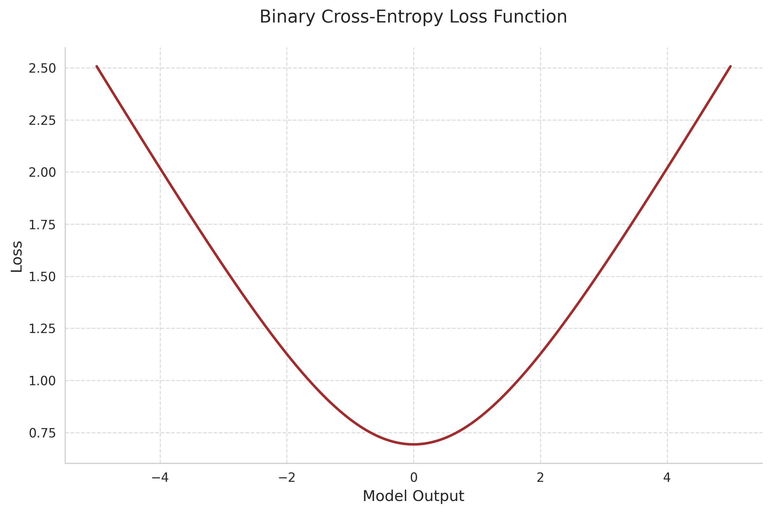
Binary cross-entropy for a binary target

L=-\frac{1}{n}\sum_i \left[y_i\log p_i+(1-y_i)\log(1-p_i)\right]

Binary cross-entropy is non-negative and unbounded above. Use it for a binary target or independently modeled multilabel targets. In training code, pass logits to a stable operation such as BinaryCrossentropy(from_logits=True) rather than manually applying sigmoid and taking logarithms.

3. Categorical Cross-Entropy

For a one-hot target $y$ and a categorical distribution $p$ :

L=-\sum_{k=1}^{K}y_k\log p_k

Use sparse categorical cross-entropy when the target is an integer class index. Softmax and categorical cross-entropy are normally combined from logits for numerical stability.

4. Focal Loss

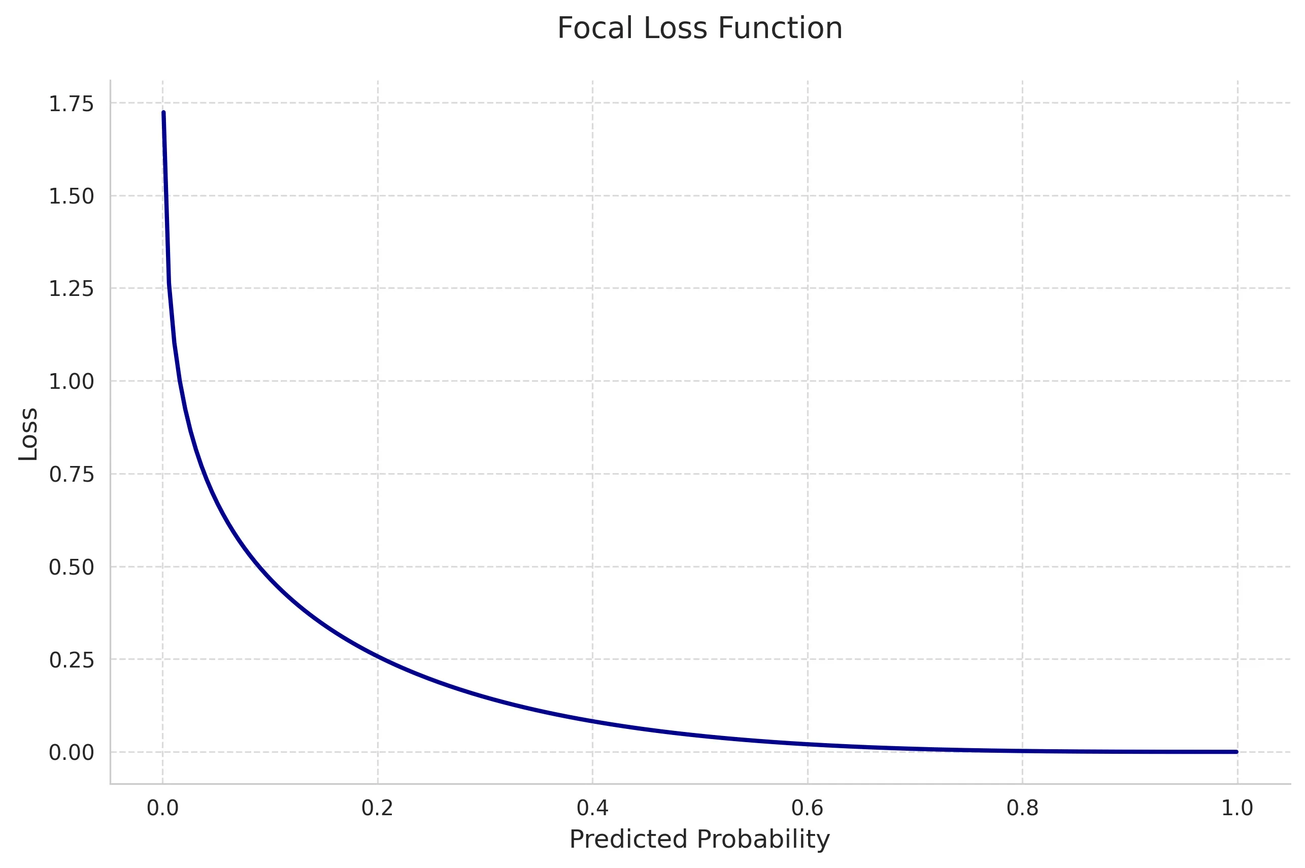
Focal loss down-weights well-classified examples

For the probability $p_t$ assigned to the true class:

\operatorname{FL}(p_t)=-\alpha_t(1-p_t)^\gamma\log(p_t)

The focusing parameter $\gamma$ reduces the contribution of well-classified examples, while $\alpha_t$ can adjust class weighting. Focal loss was introduced for dense object detection. It can help with some imbalanced datasets, but it does not automatically correct bad labels, sampling bias, probability calibration, or a mismatch between the metric and training objective.

5. Huber Loss

Let $r=\hat y-y$ . For threshold $\delta>0$ :

L_\delta(r)= \begin{cases} \frac{1}{2}r^2 & |r|\le\delta\\ \delta\left(|r|-\frac{1}{2}\delta\right) & |r|>\delta \end{cases}

The derivative with respect to the prediction is:

\frac{\partial L_\delta}{\partial\hat y}= \begin{cases} \hat y-y & |\hat y-y|\le\delta\\ \delta\,\operatorname{sign}(\hat y-y) & |\hat y-y|>\delta \end{cases}

Huber loss is quadratic near zero and linear for large residuals, so it is less sensitive to outliers than MSE. The choice of $\delta$ should reflect the scale of the target or residuals.

6. Hinge Loss

For label $y\in\{-1,1\}$ and score $s$ :

L=\max(0,1-ys)

Hinge loss trains a margin rather than a probability and is associated with support-vector machines. A score trained with hinge loss should not be presented as a calibrated probability without an additional calibration step.

TensorFlow Examples

import tensorflow as tf

x = tf.constant([-2.0, 0.0, 2.0])

relu = tf.nn.relu(x)
leaky_relu = tf.nn.leaky_relu(x, alpha=0.01)
sigmoid = tf.nn.sigmoid(x)
tanh = tf.nn.tanh(x)
softmax = tf.nn.softmax(x)
elu_alpha_1 = tf.nn.elu(x)  # tf.nn.elu fixes alpha at 1
selu = tf.nn.selu(x)
gelu = tf.nn.gelu(x)

y_true = tf.constant([[1.0], [0.0]])
logits = tf.constant([[1.2], [-0.7]])

bce = tf.keras.losses.BinaryCrossentropy(from_logits=True)
print("Binary cross-entropy:", float(bce(y_true, logits)))

predictions = tf.constant([[2.5], [-0.2]])
targets = tf.constant([[3.0], [0.0]])

print("MSE:", float(tf.keras.losses.MeanSquaredError()(targets, predictions)))
print("Huber:", float(tf.keras.losses.Huber(delta=1.0)(targets, predictions)))

For ELU with a configurable $\alpha$ , implement the two branches explicitly or use a Keras layer whose documented API exposes that parameter. Accepting an alpha argument and then calling tf.nn.elu would be misleading because tf.nn.elu uses $\alpha=1$ .

Stable NumPy softmax looks like this:

import numpy as np

def softmax(values, axis=-1):
    shifted = values - np.max(values, axis=axis, keepdims=True)
    exponentials = np.exp(shifted)
    return exponentials / np.sum(exponentials, axis=axis, keepdims=True)

Choosing the Output and Loss Together

Task	Model output	Training loss
Real-valued regression	Linear value	MSE, MAE, Huber, or a suitable likelihood
Binary classification	One logit	Binary cross-entropy from logits
Independent multilabel classification	One logit per label	Binary cross-entropy from logits
Mutually exclusive multiclass classification	One logit per class	Categorical cross-entropy from logits
Margin-based binary classification	Unbounded score	Hinge loss with $-1/+1$ targets

Hidden-layer activations such as ReLU, ELU, or GELU do not pair directly with a particular loss. The important pairing is between the output representation, target encoding, and loss.

Conclusion

Activation and loss functions are not interchangeable ingredients. Hidden activations shape gradient flow and representation; the output and loss encode what the model is claiming about its target. Choose that claim first, use a stable combined loss implementation, and check the assumptions against the data.